Whenever a baby is born, doctors measure a number of vital statistics about them: height, weight, number of fingers-and-toes, etc. A newborn child is generally considered healthy if they fall somewhere near the average in all of those categories, with a normal, healthy height and weight, and with 10 fingers-and-toes apiece. Sometimes, a child will have an unusually low or high height or weight, or greater or fewer than 10 fingers-and-toes, and the doctors will want to monitor them, ensuring that “not normal” doesn’t imply a problem. However, it turns out that there being an idea of “normal,” where “normal” means the most common set of outcomes, is universal to practically anything we dare to measure in large quantities.
It’s easy to imagine for something like height, as while there are many full grown adults of average height, there are fewer numbers of tall people and short people, and even fewer numbers of extremely tall or extremely short people. But in nature, practically anything that you measure will wind up following a Bell curve distribution, also known as a normal or Gaussian distribution. Why is that? That’s what L Viswanathan wants to know, writing in to ask:
“[I] read your recent post about [the] Fibonacci series, which prompted this question. We know that most of the phenomena in nature follow the normal distribution curve. But why? Could you please explain?”
It’s a relatively simple question, but the answer is one of great mathematical profundity. Here’s the story behind it.

The starting point, in anything that’s going to follow some sort of distribution, is what’s known as a random variable. It could be:
- whether a coin lands heads or tails,
- whether a rolled die lands on a 1, 2, 3, 4, 5, or 6,
- what your measurement error is when you measure someone’s height,
- what direction a spinner lands in when you spin it,
or many other examples. It simply refers to any case where there are multiple possible outcomes (rather than one and only one outcome) but that, when you make the measurement, you always and only get one particular answer.

It doesn’t matter what the likelihood of getting each outcome is. It doesn’t matter whether you have a fair coin or a biased coin. It doesn’t matter whether or not the die is weighted or unweighted, so long as there remains a non-zero chance of getting anything other than one option 100% of the time. And it doesn’t matter whether you have a discrete set of outcomes (e.g., a single die can only land on 1, 2, 3, 4, 5, or 6) or a continuous set of outcomes (a spinner can land on any angle from 0° to 360°, inclusive). Take enough measurements, and your sample will always follow a normal, or Bell curve, distribution.
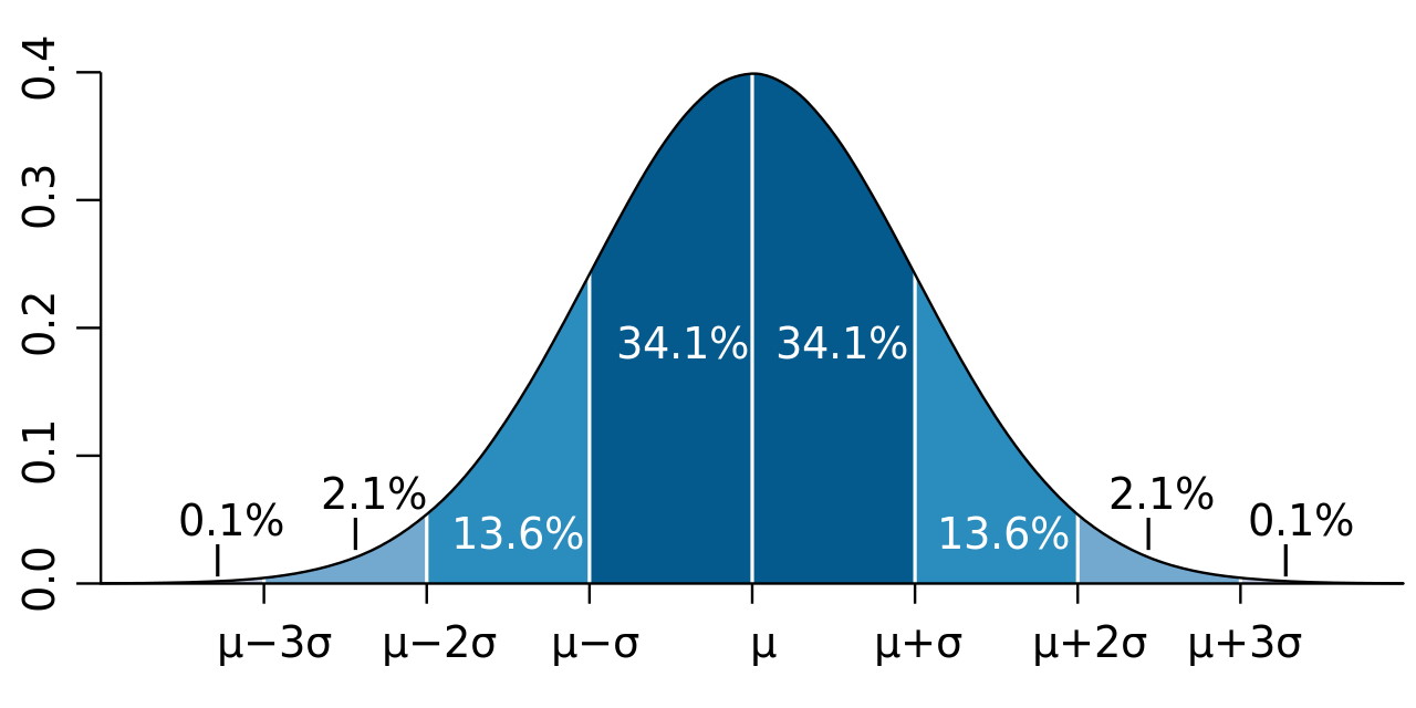
In fact, every single Bell curve (or normal distribution) that exists can be shown, mathematically, to simply be a rescaled version of the standard normal distribution. The only rescalings that ever need to occur are:
- a rescaling of the average value of the domain (x-axis, or the thing you’re measuring) so that the central value winds up representing the mean value (µ) of your outcomes,
- a rescaling of the range of the domain (x-axis, which is again the thing you’re measuring) to reflect the standard deviation (σ) of your distribution,
- and, finally, a rescaling of the probability density (y-axis, or the frequency of how likely you are to arrive at this particular outcome) so that the total area under the Bell curve equals 1, signifying a 100% probability that one of the outcomes represented by your probability graph will occur.
This means that if you measure the heights of 1000 different adults of the same gender, you’ll get a normal distribution, with an average value (µ) and a standard deviation (σ) that reflects the height distribution of your sample, whose total probability adds up to 100%. It also means that if, instead, you measure your own height 1000 different times, you’ll get an average value for your own height (a different µ), along with a standard deviation (a different σ) that reflects your measurement uncertainty in measuring your own height, where the total probability again adds up to 100%. Bell curves (or normal distributions) can be wide or narrow, but can always be rescaled to give precisely the same shaped curve.

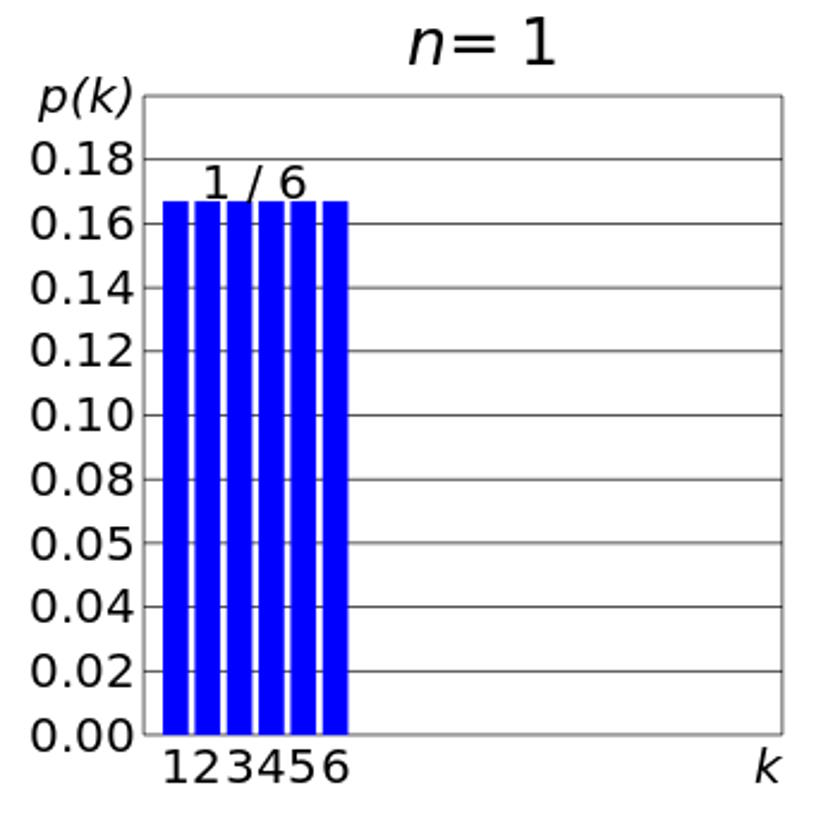
It’s not immediately obvious, however, that pretty much everything in nature that can be measured will show a normal distribution when you consider the outcomes that can occur. Consider a fair, six-sided die, for example. Before you roll it once, you know that there are going to be six possible outcomes for this die, and you know furthermore, assuming the die roll is fair, what the odds are of getting each of those outcomes. They are as follows:
- 1: 1-in-6,
- 2: 1-in-6,
- 3: 1-in-6,
- 4: 1-in-6,
- 5: 1-in-6, and
- 6: 1-in-6.
That means there is a 16.666% chance of getting either a 1, 2, 3, 4, 5, or 6 with your die roll, with no other outcomes possible.
If you were to graph these possibilities out, you would immediately see, plain as day, that this didn’t appear to follow a normal distribution, or Bell curve, but instead appeared to be a completely flat distribution that didn’t favor getting the mean, or average, value (something like a 3 or a 4) over one of the more extreme values (something like a 1 or a 6). That’s because although a single die roll is a random variable, it’s not what we call a Gaussian random variable: it doesn’t have the normal distribution inherent to any single outcome.
But now, let’s jump ahead another step: what if instead of rolling one fair six-sided die, we rolled two fair six-sided dice? Sure, for each individual die, they have the same probabilities that they did previously, with a 16.666% chance of each one giving either a 1, 2, 3, 4, 5, or 6, equally. If you ever need to place a bet on the outcome of any one fair six-sided die, that’s going to be the case for what you expect the outcome of the die roll to be.
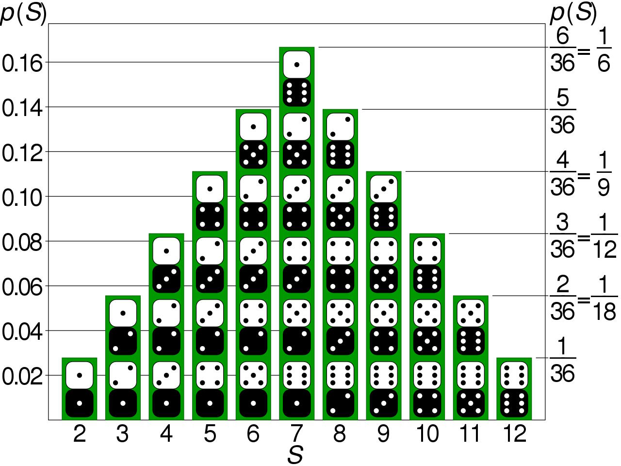
However, when we roll two dice together, we no longer see a flat distribution in the set of possible outcomes, but note that it starts to look a little more like a Bell curve. If you roll two six-sided dice in tandem, your outcomes, and the odds associated with them, are:
- 2: 1-in-36,
- 3: 1-in-18 (2-in-36),
- 4: 1-in-12 (3-in-36),
- 5: 1-in-9 (4-in-36),
- 6: 1-in-7.2 (5-in-36),
- 7: 1-in-6 (6-in-36),
- 8: 1-in-7.2 (5-in-36),
- 9: 1-in-9 (4-in-36),
- 10: 1-in-12 (3-in-36),
- 11: 1-in-18 (2-in-36), and
- 12: 1-in-36.
Just by taking two examples of a random variable that had an initially flat distribution, we’re now getting much closer to seeing a Bell curve, or normal distribution, begin to emerge from it.
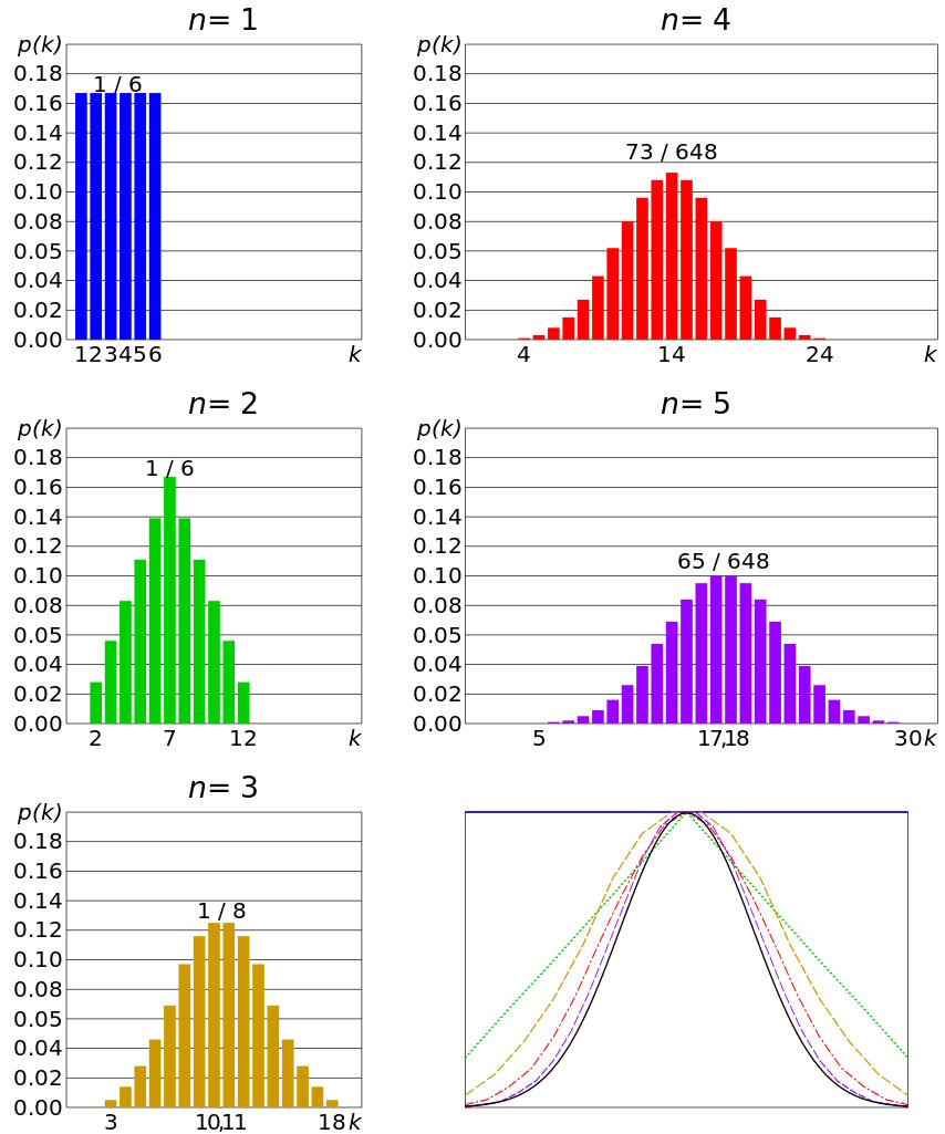
You can, in fact, get closer and closer to a Bell curve (normal distribution) simply by taking more and more instances of a random variable like a dice roll. If you roll three six-sided dice together, you’re much more likely to get a value close to the mean (10.5) than you are to get a value far away from the mean (such as 3 or 18, to the chagrin of Dungeons & Dragons players everywhere). If you continue to increase the number of dice you roll — to four, five, or six, for example — it’s going to be more and more difficult to wind up at the extreme ends of the distribution: to roll exclusively all low or all high numbers.
Instead, you’re going to be more likely to see a mix of values in your dice rolls: where some numbers are high, some numbers are low, and some numbers are in-between, giving you a value that isn’t necessarily going to be precisely at the mean value, but rather a value that’s most likely to be within some “range” of the mean value. You’ll be less likely, but still not super unlikely, to get a value that’s slightly farther away from the mean value: within a wider range around it. But the farther away from the mean you’re willing to look, the less and less likely it becomes that you’re going to achieve such a value with more and more samples. That’s the kind of trial work that’s going to reproduce a Bell curve, or a normal distribution, the more samples you take.
You might wonder about an extreme example that very, very clearly doesn’t have a Gaussian random variable underlying it: the binomial distribution. This special case occurs when you have only two outcomes that are possible, and oftentimes, each of those two outcomes are equally likely, such as the “heads or tails” nature of a fair coin flip.
If you flip only one coin, you’re going to get either “heads” or “tails,” despite the fact that the average value of all possible outcomes is “half-heads and half-tails,” which occurs absolutely 0% of the time for a single flipped coin.
But now, imagine flipping two coins. Sure, there’s a 1-in-4 chance of you getting two heads, and a 1-in-4 chance of you getting two tails, but this time, just by adding a second coin into the mix, now there’s a 1-in-2 (or 50%) chance that you get 1 heads and 1 tails for your coins, which is precisely the average value of “half-heads and half-tails.”
If you were to flip ever greater numbers of coins — and assigned a value of “0” to every tails and a value of “1” to every heads — you would find very quickly that the average value for your flipped coins came out to 0.5: half-heads and half-tails. There would be a normal distribution around that average value, and the more “flips” there were, the smaller the standard deviation (or “width”) you’d see to your normal distribution.
This works, in fact, for any binomial distribution, even if the odds aren’t “50:50” of having one outcome or the other, but any split odds you like. And this isn’t just an approximate property that emerges, but rather a proven mathematical theorem that dates all the way back to the 18th century, when French mathematician Abraham de Moivre derived it and published it in the 2nd edition of his 1738 book The Doctrine of Chances. Today, it’s known as the de Moivre-Laplace theorem, and it tells you that:
- if you have n trials,
- where each trial has a probability p of success,
- then you’ll wind up with a normal distribution for your set of outcomes,
- where the mean (average) value is np,
- and the standard deviation to your Bell curve will be √(np(1-p)),
as long as p is not equal to 0 or 1, meaning it’s not a “rigged” trial that will be either 0% or 100% successful.
The greater the number of trials you use, in fact, the closer the distribution of outcomes mirrors the normal distribution, and, just like before, the narrower the “peak” of your distribution becomes, with the standard deviation getting smaller and smaller relative to the total number of trials that you run.
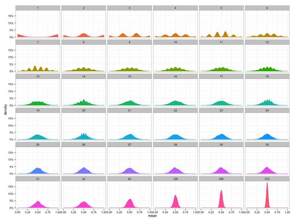
It turns out that examples like “starting out with Gaussian random variables” or “rolling the dice” or “flipping large numbers of coins” or even the more general “de Moivre-Laplace theorem” are only special cases of a more general theorem in mathematics that came to the forefront in the early 20th century: the central limit theorem. It says, in a general sense, that:
- if you have some sort of sample,
- and you seek to measure a variable within that sample,
- that by measuring that variable across a great number of members of that sample,
- you will wind up seeing approximately a normal distribution,
- even under nearly all conditions,
- even if the variables are not random and/or independent,
- and that you will more accurately approximate a normal distribution, even in the low-probability tails, by taking ever-greater numbers of members of the sample.
Mathematically, you can see this illustrated with a number of examples that reflect a bizarre set of initial underlying probabilities, and yet, a normal distribution with a large enough sample still emerges. Many mathematicians worked together so that, by 1937, a stronger version of that theorem, the generalized central limit theorem, could be published. In physics, this has an enormous number of applications, including — perhaps quite famously — for the velocity of atoms or molecules in a gas, noting that they “relax” to follow a Maxwell-Boltzmann distribution after being allowed to interact for only a short period of time.

It’s interesting to note that this insight — that any random variable, if you sample it enough times, will produce a normal (Bell curve) distribution — was not appreciated by mathematicians or scientists for long periods of time. According to mathematician Henk Tijms, writing in his book Understanding Probability:
“The first version of [the central limit] theorem was postulated by the French-born mathematician Abraham de Moivre who, in a remarkable article published in 1733, used the normal distribution to approximate the distribution of the number of heads resulting from many tosses of a fair coin. This finding was far ahead of its time, and was nearly forgotten until the famous French mathematician Pierre-Simon Laplace rescued it from obscurity in his monumental work Théorie analytique des probabilités, which was published in 1812. Laplace expanded De Moivre’s finding by approximating the binomial distribution with the normal distribution. But as with De Moivre, Laplace’s finding received little attention in his own time. It was not until the nineteenth century was at an end that the importance of the central limit theorem was discerned, when, in 1901, Russian mathematician Aleksandr Lyapunov defined it in general terms and proved precisely how it worked mathematically. Nowadays, the central limit theorem is considered to be the unofficial sovereign of probability theory.”
In other words, irrespective of:
- how a variable behaves,
- whether there are one, several, or many variables,
- whether they are interrelated or completely independent,
- whether there are two, several, or infinitely many outcomes,
- and whether all outcomes are equally likely or whether there’s a weight to their distribution,
if you sample that variable enough times, you’re pretty much always going to wind up with a normal, Bell curve-like distribution for your outcomes. There will be a mean value, a standard deviation, and a total probability of 100% that you arrive at in the end, and that’s not even a function of something going on in nature, but a simple fact of pure mathematics.
Send in your Ask Ethan questions to startswithabang at gmail dot com!

The Power of Play