The reality of quantum fluctuations was proven back in 1947

If you spend enough time listening to theoretical physicists, it starts to sound like there are two separate worlds that they inhabit.

1. The real, experimental-and-observational world, full of quantities and properties we can measure to high precision with a sufficient setup.
2. The theoretical world that underlies it, full of esoteric calculational tools that model reality, but can only describe it in mathematical, rather than purely physical, terms.

One of the most glaring examples of this is the idea of virtual particles. In theory, there are both the real particles that exist and can be measured in our experiments, and also the virtual particles that exist throughout all of space, including empty space (devoid of matter) and occupied (matter-containing) space. The virtual ones do not appear in our detectors, don’t collide with real particles, and cannot be directly seen. As theorists, we often caution against taking the analogy of virtual particles too seriously, noting that they’re just an effective calculational tool, and that there are no actual “pairs” of particles that pop in-and-out of existence in our lived reality.

However, virtual particles do affect the real world in important, measurable ways, and in fact their effect was first discovered way back in 1947, before theorists were even aware of how necessary they were. Here’s the remarkable story of how we proved that quantum fluctuations must be real and have real effects on our measured world, even before we understood the theory behind them.

Hydrogen nuclei come in three varieties: with a single proton for its nucleus, which is stable, with a proton and neutron bound together, known as a deuteron, which is stable, and with a single proton and two neutrons, known as a triton, which radioactively decays with a half-life of 12 years. The binding energy in a deuteron will keep it stable; the binding energy in a triton will not. Over 99.9% of all hydrogen atoms in the Universe have only a simple proton for their nucleus.

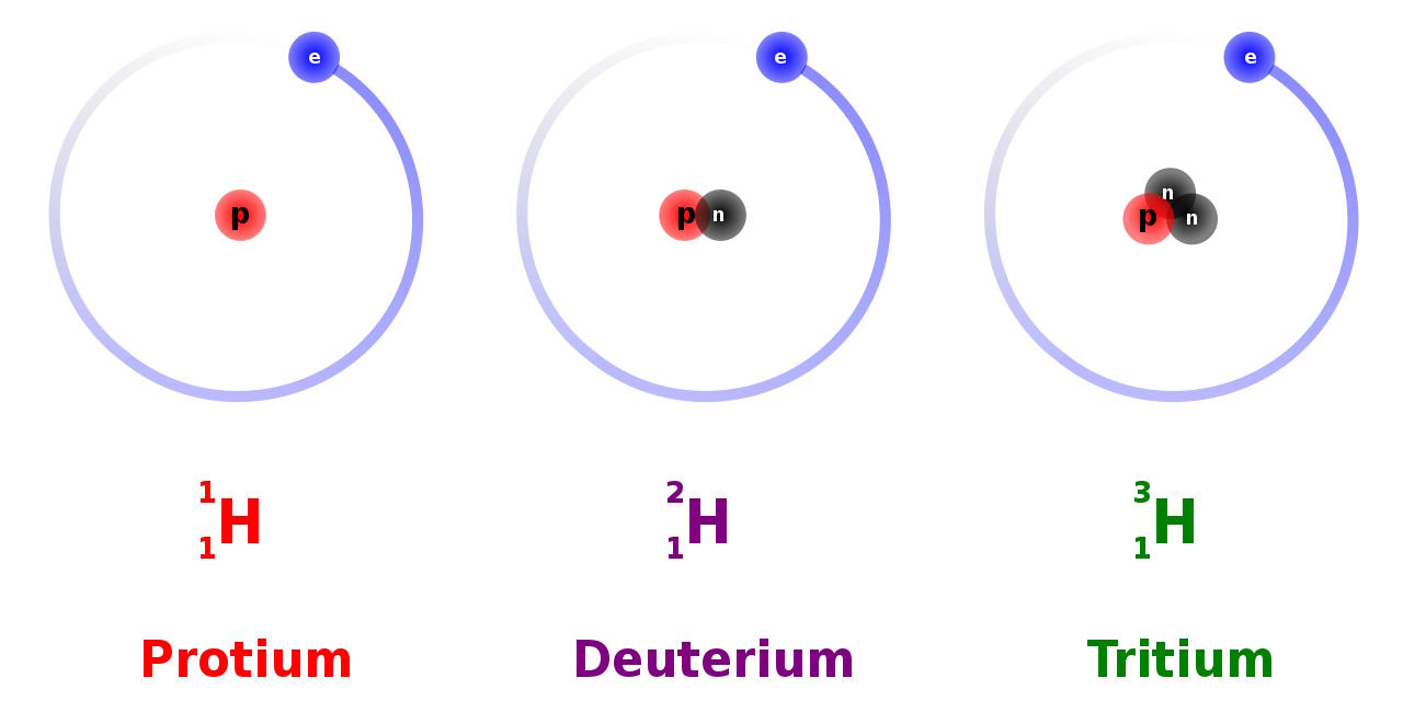
Imagine the simplest atom of all: the hydrogen atom. This was, in many ways, the “proving ground” for quantum theory, as it’s one of the simplest systems in the Universe, made up of one positively charged proton with an electron bound to it. Yes, the proton is complicated, as it itself is made of quarks and gluons bound together, but for the purposes of atomic physics, it can frequently be treated as a point particle with a few quantum properties:

• a mass (about 1836 times heavier than the electron’s mass),
• an electric charge (positive, and equal and opposite to the electron’s charge),
• and a half-integer spin (either +½ or -½), or an intrinsic amount of angular momentum (in units of Planck’s constant, ħ).

When an electron binds to a proton, it forms a neutral hydrogen atom, with the entire system having a slightly smaller amount of rest mass than the free proton and free electron combined. If you put a neutral hydrogen atom on one side of a scale and a free electron and free proton on the other size, you’d find the neutral atom was lighter by about 2.4 × 10^-35 kg: a minuscule amount, but a very important one nonetheless.

This artist’s illustration shows an electron orbiting an atomic nucleus, where the electron is a fundamental particle but the nucleus can be broken up into still smaller, more fundamental constituents. The simplest atom of all, hydrogen, is an electron and a proton bound together. Other atoms have more protons in their nucleus, with the number of protons defining the type of atom we’re dealing with. Electrons and atomic nuclei that are bound together into neutral atoms have slightly less mass than free electrons and nuclei in unbound states.

That tiny difference in mass comes from the fact that when protons and electrons bind together, they emit energy. That emitted energy comes in the form of one-or-more photons, as there are only a finite number of explicit energy levels that are allowed: the energy spectrum of the hydrogen atom. As an initially excited electron cascades down through the various energy levels, culminating in a transition down to (eventually) the lowest-energy state allowed — known as the ground state — photons are released, with the energy, frequency, and wavelength of that photon determined by the different energy levels that the electron occupies before-and-after the transition.

If you were to capture all of the photons emitted during a transition from a free proton and a free electron down to a ground state hydrogen atom, you’d find that the exact same amount of total energy was always released: 13.6 electron-volts, or an amount of energy that would raise the electric potential of one electron by 13.6 volts. That energy difference is exactly the mass-equivalence of the difference between a free electron and proton versus a bound, ground state hydrogen atom, which you can calculate yourself from Einstein’s most famous equation: E = mc².

The differences in electron energy levels occur in all atoms, from the simplistic hydrogen to the most complex elements of all. This graph illustrates the energy level differences in an atom of Lutetium-177. Note how there are only specific, discrete energy levels that are acceptable. While the energy levels are discrete, the positions of the electrons are not.

According to the quantum rules that govern the Universe, a bound electron in an atom is very different than a free electron.

• Whereas a free electron can carry any amount of energy at all, a bound electron can only carry a few explicit, specific amounts of energy within an atom.
• Whereas free electrons are allowed to move in any direction at all with any momentum at all, the possibilities for a bound electron are restricted by a set of quantum rules.
• And a free electron’s energy possibilities are continuous, while a bound electron’s energy possibilities are discrete, and can only take on specific values.

In fact, the reason we call it “quantum physics” comes exactly from this phenomenon: the energy levels a bound particle can occupy are quantized, and can only come in specific quantities that obey the mathematical rules that bound states mandate.

However, an electron in the ground state — remember, the lowest-energy state — won’t be in a specific place at a specific time, like a planet orbiting a star would be. Instead, it makes more sense to calculate the probability distribution of the electron: the odds, averaged over space and time, of finding it in a particular location at any particular moment. Remember that quantum physics is inherently unlike classical physics: instead of being able to measure exactly where a particle is and how it’s moving, you can only know the combination of those two properties to some specific, limiting precision. Measuring one more precisely inherently leads to knowing the other less precisely.

This diagram illustrates the inherent uncertainty relation between position and momentum. When one is known more accurately, the other is inherently less able to be known accurately. Both position and momentum are better described by a probabilistic wavefunction than by a single value. Other pairs of conjugate variables, including energy and time, spin in two perpendicular directions, or angular position and angular momentum, also exhibit this same uncertainty relation.

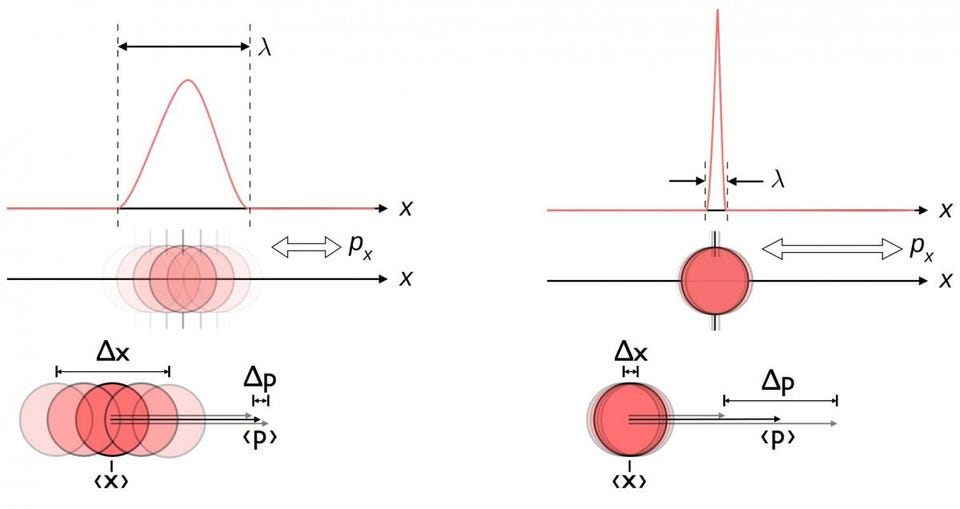
As a result, we do better to think of an electron not as a particle when it’s in a hydrogen atom, but rather as a “probability cloud” or some other, similarly fuzzy visualization. For the lowest-energy state, the probability cloud of an electron looks like a sphere: you’re most likely to find it an intermediate distance away from the proton, but you’ve got a non-zero probability of finding it very far away or even at the center: within the proton itself. Until you make a critical measurement, however, it’s more accurate to describe the electron’s properties probabilistically: occupying a set of values with a particular set of probability amplitudes, rather than having a specific position and momentum at any moment in time.

In other words, it isn’t the position of the electron at any moment in time that determines its energy; rather, it’s the energy level the electron occupies that determines the relative probabilities of where you’re most and least likely to find that electron any time you make a measurement.

There is a relationship, though, between the average distance you’re likely to find the electron at from the proton and the energy level of the electron within the atom. This was the big discovery of Niels Bohr: that the electron occupies discrete energy levels that correspond to, in his simplified model, being multiples of a specific distance from the nucleus.

Electron transitions in the hydrogen atom, along with the wavelengths of the resultant photons, showcase the effect of binding energy and the relationship between the electron and the proton in quantum physics. The Bohr model of the atom provides the coarse (or rough, or gross) structure of these energy levels. Hydrogen’s strongest transition is Lyman-alpha (n=2 to n=1), but its second strongest is visible: Balmer-alpha (n=3 to n=2), which emits visible (red) light at a wavelength of 656 nanometers. The energy lost by an electron cascading down the energy levels gets emitted in the form of photons.

Bohr’s model works incredibly well for determining the energies of transitions between the various levels of the hydrogen atom that the electron can occupy. If you have an electron in the first excited state, it can transition down to the ground state, emitting a photon in the process. The ground state has only one possible orbital that the electrons can occupy: the 1S orbital, which is spherically symmetric. That orbital can hold up to two electrons: one with spin +½ and one with spin -½, either aligned or anti-aligned with the proton’s spin. There are no other possibilities for an electron in the ground (1st energy level) state of the hydrogen atom.

But when you jump up to the first excited state, there are now multiple orbitals the electrons can occupy, corresponding to the arrangement most of us are familiar with on the periodic table.

• Electrons can occupy the 2S orbital, which is spherically symmetric but has a mean distance that is double the 1S orbital’s, and has various radii of high-and-low probabilities.
• Additionally, however, electrons can also occupy the 2P orbital, which is divided into three perpendicular directions corresponding to three dimensions: the x, y, and z directions. Again, the mean distance of the electron from the nucleus is double the 1S orbital’s.

The lowest energy level (1S) of hydrogen (top left) has a dense electron probability cloud. Higher energy levels have similar clouds, but with much more complicated configurations and covering a much larger volume of space. For the first excited state, there are two independent configurations: the 2S state and the 2P state, which have different energy levels due to a very subtle quantum effect.

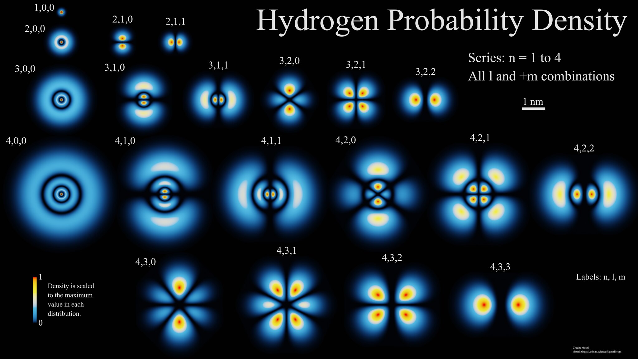
These energy levels were known way before Bohr’s 1913 model, going way back to Balmer’s 1885 work on spectral lines. By 1928, Dirac had put forth the first relativistic theory of quantum mechanics that included the electron and the photon, showing that — at least theoretically — there should be corrections to those energy levels if they had different spin or orbital angular momenta between them: corrections that were experimentally determined between, for instance, the various 3D and 3P orbitals. (You can see this visually in the image above, as 3,1,0 and 3,1,1 correspond to the 3P orbitals, while 3,2,0, 3,2,1 and 3,2,2 correspond to the 3D orbitals.)

However, in both Bohr’s and Dirac’s theory, electrons in the 2S orbital and the 2P orbital should have the same energies. Do they? We didn’t know for decades, as this wasn’t measured until a very clever experiment came along in 1947, conducted by Willis Lamb and Robert Retherford.

What they did was prepare a beam of hydrogen atoms in the ground (1S) state, and then hit that beam with electrons that bump some of the atoms up to the 2S state. Under normal circumstances, these 2S electrons take a long time (a few hundred milliseconds) to transition back to the 1S state, since you have to emit two photons (instead of just one) to prevent your electron from undergoing a forbidden spin transition. Alternatively, you can collide those excited atoms with a piece of tungsten foil, which causes the atoms with 2S electrons to de-excite, emitting detectable radiation.

In the Lamb-Retherford experiment, electrons are excited by a beam from the 1S state into the 2S state, then pumped with photons at a tuned frequency until many enter the 2P state. The effects can be seen at the detector, which is a thin piece of tungsten foil, sensitive to 2S electrons but not 2P or 1S electrons. The effect of the additional ~1 GHz photons show the effect of the Lamb shift.

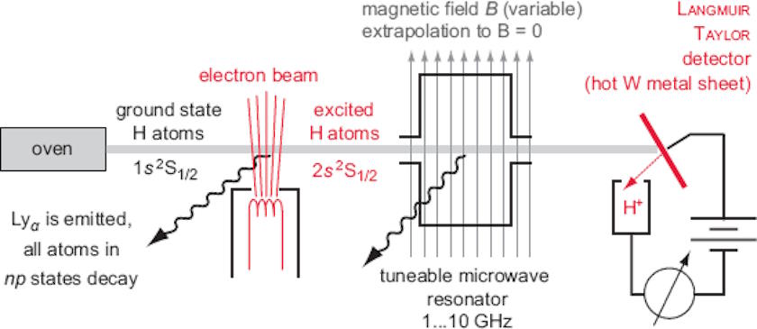
On the other hand, electrons in the 2P state should transition much more quickly: in about ~1 nanosecond, since they only need to emit one photon for the quantum transition and there are no quantum rules forbidding the emission of one such photon. The clever trick that Lamb and Retherford used was to add in a resonator that could be tuned, bombarding the now-excited electrons with electromagnetic radiation. When the electromagnetic frequency reached just a tiny bit over 1 GHz, some of the excited hydrogen atoms started emitting photons right away (within nanoseconds), de-exciting back to the 1S state.

The immediate drop in the detectable radiation at the right frequency was an enormous surprise, providing strong evidence that these atoms had been excited into the 2P state, rather than the 2S state.

Think about what that means: without this additional radiation, the excited electrons would only go into the 2S state, never the 2P state. Only with the addition of energy-carrying radiation could the electrons be coaxed from the 2S state into the 2P state. That means that the additional radiation must be getting absorbed by the electrons, and that the additional absorption of energy “bumps them up” from the 2S state into the 2P state.

In the Bohr model of the hydrogen atom, only the orbiting angular momentum of the point-like electron contributes to the energy levels. Adding in relativistic effects and spin effects not only causes a shift in these energy levels, but causes degenerate levels to split into multiple states, revealing the fine structure of matter atop the coarse structure predicted by Bohr.

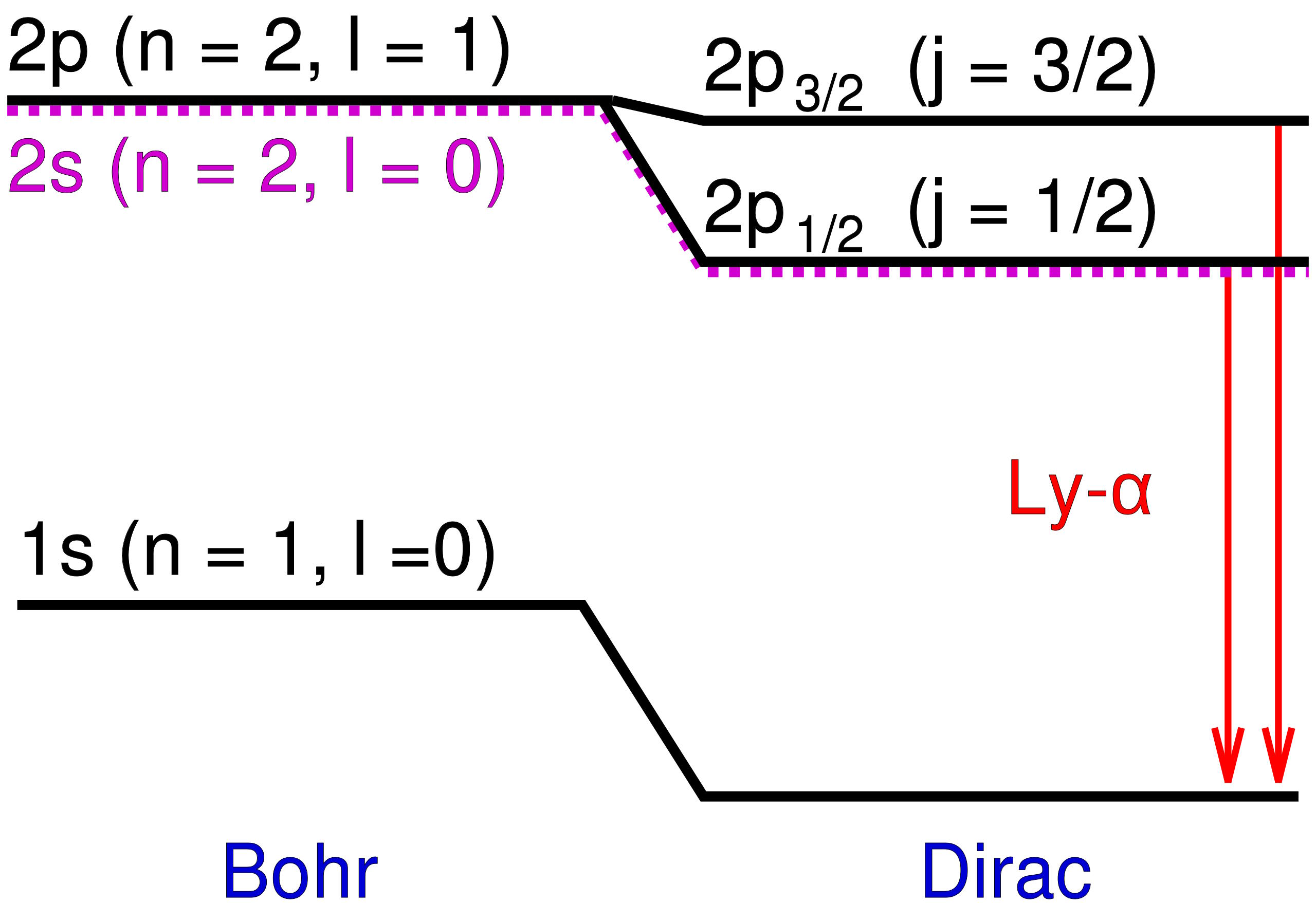
The implication, if you haven’t realized it yet, is astounding. Despite the predictions of Bohr, Dirac, and quantum theory as we understood it, the 2P state didn’t have the same energy as the 2S state. The 2P state has a slightly higher energy — known today as the Lamb shift — an experimental fact that the work of Lamb and Retherford clearly demonstrated. What wasn’t immediately clear was why this is the case.

Some thought it could be caused by a nuclear interaction; that was shown to be wrong. Others thought that the vacuum might become polarized, but that was also wrong.

Instead, as was first shown by Hans Bethe later that year, this was due to the fact that all of an atom’s energy levels are shifted by the interaction of the electron with what he called “the radiation field,” which can only be accounted for properly in a quantum field theory, such as quantum electrodynamics. The resulting theoretical developments brought about modern quantum field theory, and the interactions with virtual particles — the modern way to quantify the effects of “the radiation field” — provide the exact effect, including the right sign and magnitude, that Lamb measured back in 1947.

There is a non-zero energy inherent to quantum fields themselves: including the radiation field from electrodynamics, the chromodynamic field from the strong nuclear force, and the weak field from the weak nuclear force. These manifest, in our calculations, as virtual particles which appear in Feynman diagrams. They cannot be ignored, and their effect was first measured before they were predicted: in 1947, via the Lamb shift.

The results of the Lamb-Retherford experiment are sufficient to prove the existence of the very real effects of quantum fluctuations. We can conceptualize it like this: the atom itself is always present, and it exerts an electromagnetic force, the Coulomb force, which governs electrostatic attraction. The quantum fluctuations in the electromagnetic field cause electron fluctuations in its position, and that causes the average Coulomb force to be slightly different from what it would be without these quantum fluctuations. Because the geometry of the 2S and 2P orbitals are slightly different from one another, those quantum fluctuations — which show up as virtual photons from the charged particles in the atom — affect the orbitals differently, resulting in the physical phenomenon known, today, as the Lamb shift.

To be sure, there are definitely going to be differences between the shift of a bound electron and the shift of a free electron, but even free electrons are destined to interact with the quantum vacuum. No matter where you go, you cannot escape the quantum nature of the Universe. Today, the hydrogen atom is one of the most stringent testing grounds for the rules of quantum physics, giving us a measurement of the fine structure constant — α — to better than 1-part-in-1,000,000. The quantum nature of the Universe extends not only to particles, but to fields as well. It isn’t just theory; our experiments have demonstrated this unavoidable reality for more than three-quarters of a century.